new

% Defining the periodic signals T = 2*pi; % Period of the signal t = linspace(-T, T, 1000);

% Number of harmonics to compute N = 10;

% Initialize coefficient arrays a_0 = 0; % DC Component

% Initialize coefficient arrays for each signal a_n_square = zeros(1, N); b_n_square = zeros(1, N); a_n_sawtooth = zeros(1, N); b_n_sawtooth = zeros(1, N); a_n_sine = zeros(1, N); b_n_sine = zeros(1, N); a_n_cosine = zeros(1, N); b_n_cosine = zeros(1, N);

% Define and analyze square wave signal = square(t); for n = 1:N a_n_square(n) = (2/T) * trapz(t, signal .* cos(n * (2pi/T) * t)); b_n_square(n) = (2/T) * trapz(t, signal . sin(n * (2*pi/T) * t)); end

% Define and analyze sawtooth wave signal = sawtooth(t, 0.5); for n = 1:N a_n_sawtooth(n) = (2/T) * trapz(t, signal .* cos(n * (2pi/T) * t)); b_n_sawtooth(n) = (2/T) * trapz(t, signal . sin(n * (2*pi/T) * t)); end

% Define and analyze sine wave signal = sin(t); for n = 1:N a_n_sine(n) = (2/T) * trapz(t, signal .* cos(n * (2pi/T) * t)); b_n_sine(n) = (2/T) * trapz(t, signal . sin(n * (2*pi/T) * t)); end

% Define and analyze cosine wave signal = cos(t); for n = 1:N a_n_cosine(n) = (2/T) * trapz(t, signal .* cos(n * (2pi/T) * t)); b_n_cosine(n) = (2/T) * trapz(t, signal . sin(n * (2*pi/T) * t)); end

% Display results for each signal disp(‘Fourier Series Coefficients for Square Wave:’) disp([‘a_0: ’, num2str(a_0)]) for n = 1:N disp([num2str(n), ’ ’, num2str(a_n_square(n)), ’ ’, num2str(b_n_square(n))]); end

disp(‘Fourier Series Coefficients for Sawtooth Wave:’) disp([‘a_0: ’, num2str(a_0)]) for n = 1:N disp([num2str(n), ’ ’, num2str(a_n_sawtooth(n)), ’ ’, num2str(b_n_sawtooth(n))]); end

disp(‘Fourier Series Coefficients for Sine Wave:’) disp([‘a_0: ’, num2str(a_0)]) for n = 1:N disp([num2str(n), ’ ’, num2str(a_n_sine(n)), ’ ’, num2str(b_n_sine(n))]); end

disp(‘Fourier Series Coefficients for Cosine Wave:’) disp([‘a_0: ’, num2str(a_0)]) for n = 1:N disp([num2str(n), ’ ’, num2str(a_n_cosine(n)), ’ ’, num2str(b_n_cosine(n))]); end

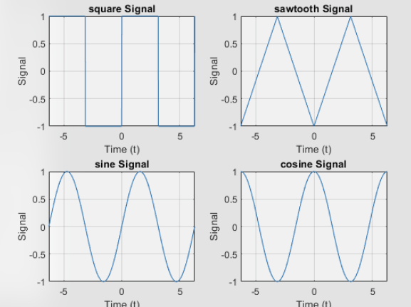
% Plot the original signals figure; subplot(2,2,1); plot(t, square(t)); title(‘Square Wave’); xlabel(‘Time (t)’); ylabel(‘Signal’); grid on;

subplot(2,2,2); plot(t, sawtooth(t, 0.5)); title(‘Sawtooth Wave’); xlabel(‘Time (t)’); ylabel(‘Signal’); grid on;

subplot(2,2,3); plot(t, sin(t)); title(‘Sine Wave’); xlabel(‘Time (t)’); ylabel(‘Signal’); grid on;

subplot(2,2,4); plot(t, cos(t)); title(‘Cosine Wave’); xlabel(‘Time (t)’); ylabel(‘Signal’); grid on;

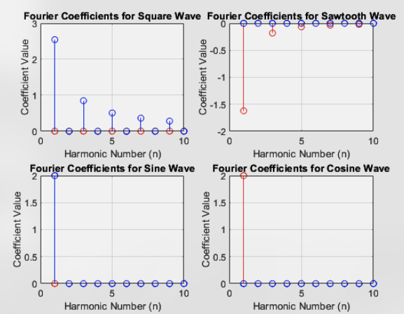
% Plot Fourier coefficients figure; subplot(2,2,1); stem(1:N, a_n_square, ‘r’, ‘DisplayName’, ‘a_n (cosine)’); hold on; stem(1:N, b_n_square, ‘b’, ‘DisplayName’, ‘b_n (sine)’); title(‘Fourier Coefficients for Square Wave’); xlabel(‘Harmonic Number (n)’); ylabel(‘Coefficient Value’); grid on;

subplot(2,2,2); stem(1:N, a_n_sawtooth, ‘r’, ‘DisplayName’, ‘a_n (cosine)’); hold on; stem(1:N, b_n_sawtooth, ‘b’, ‘DisplayName’, ‘b_n (sine)’); title(‘Fourier Coefficients for Sawtooth Wave’); xlabel(‘Harmonic Number (n)’); ylabel(‘Coefficient Value’); grid on;

subplot(2,2,3); stem(1:N, a_n_sine, ‘r’, ‘DisplayName’, ‘a_n (cosine)’); hold on; stem(1:N, b_n_sine, ‘b’, ‘DisplayName’, ‘b_n (sine)’); title(‘Fourier Coefficients for Sine Wave’); xlabel(‘Harmonic Number (n)’); ylabel(‘Coefficient Value’); grid on;

subplot(2,2,4); stem(1:N, a_n_cosine, ‘r’, ‘DisplayName’, ‘a_n (cosine)’); hold on; stem(1:N, b_n_cosine, ‘b’, ‘DisplayName’, ‘b_n (sine)’); title(‘Fourier Coefficients for Cosine Wave’); xlabel(‘Harmonic Number (n)’); ylabel(‘Coefficient Value’); grid on;