Probability & Statistics Lab 2
INFO
Visual Outputs of data in R studio File for documentation and questions P2_DATAFRAMES IN R AND DATA IMPORTING.pdf
Example Run
Write a color vector using 5 vectors and analyze cancer levels
# Load the 'cancer.csv' file into the variable 'csv'
csv = read.csv("C:\\Users\\TJ\\R Studio\\Lab 2\\cancer.csv")

# Create a vector 'vector_color' containing a list of color names.
# This will be used to categorize items into different color groups.
vector_color = c("red", "yellow", "blue", "red", "yellow", "blue", "red", "yellow", "blue", "magenta")

# Convert the 'vector_color' into a factor variable.
# A factor is used to represent categorical data in R. This function assigns levels to the color values.
colorfac = factor(vector_color)

# Get the number of unique levels in the 'colorfac' factor.
# This will tell us how many distinct categories (colors) are present in the vector.
nlevels(colorfac)

# Display a summary of the 'colorfac' factor variable.
# The summary will show the count of each color in the 'vector_color' list.
summary(colorfac)

# Convert the 'treatment' column from the 'csv' dataset into a factor.
# Assuming 'treatment' represents a categorical variable in the dataset,
# we are creating a factor variable to handle the data efficiently.
csvfactor = factor(csv$treatment)

# Display a summary of the 'csvfactor' factor variable.
# This will show us how many instances of each treatment type are in the dataset.
summary(csvfactor)

# Convert the 'cancerlevel' column from the 'csv' dataset into a factor.
# 'cancerlevel' might represent the stage or severity of cancer,
# and we are converting it into a factor variable to treat it as categorical data.
cancerlevel = factor(csv$cancerlevel)

# Display a summary of the 'cancerlevel' factor variable.
# This will show us how many instances of each cancer level are in the dataset.
summary(cancerlevel)
Output
> # Load the 'cancer.csv' file into the variable 'csv'
> csv = read.csv("C:\\Users\\TJ\\R Studio\\Lab 2\\cancer.csv")
> > # Create a vector 'vector_color' containing a list of color names.
> # This will be used to categorize items into different color groups.
> vector_color = c("red", "yellow", "blue", "red", "yellow", "blue", "red", "yellow", "blue", "magenta")
> > # Convert the 'vector_color' into a factor variable.
> # A factor is used to represent categorical data in R. This function assigns levels to the color values.
> colorfac = factor(vector_color)
> > # Get the number of unique levels in the 'colorfac' factor.
> # This will tell us how many distinct categories (colors) are present in the vector.
> nlevels(colorfac)
[1] 4
> > # Display a summary of the 'colorfac' factor variable.
> # The summary will show the count of each color in the 'vector_color' list.
> summary(colorfac)
   blue magenta     red  yellow
      3       1       3       3
> > # Convert the 'treatment' column from the 'csv' dataset into a factor.
> # Assuming 'treatment' represents a categorical variable in the dataset,
> # we are creating a factor variable to handle the data efficiently.
> csvfactor = factor(csv$treatment)
> > # Display a summary of the 'csvfactor' factor variable.
> # This will show us how many instances of each treatment type are in the dataset.
> summary(csvfactor)
 A  B  C  D
12 12 12 12
> > # Convert the 'cancerlevel' column from the 'csv' dataset into a factor.
> # 'cancerlevel' might represent the stage or severity of cancer,
> # and we are converting it into a factor variable to treat it as categorical data.
> cancerlevel = factor(csv$cancerlevel)
> > # Display a summary of the 'cancerlevel' factor variable.
> # This will show us how many instances of each cancer level are in the dataset.
> summary(cancerlevel)
 1  2  3
16 16 16
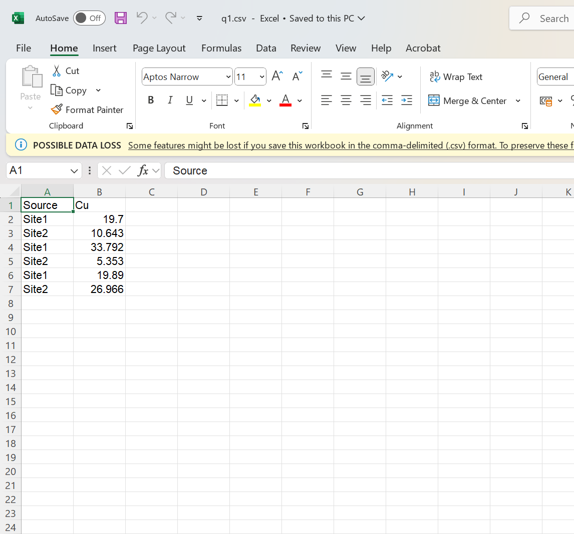
Question 1
Code
read.csv("C:\\Users\\TJ\\R Studio\\Lab 2\\q1.csv")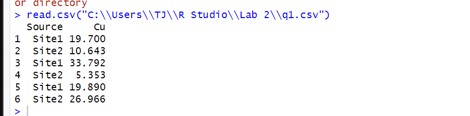
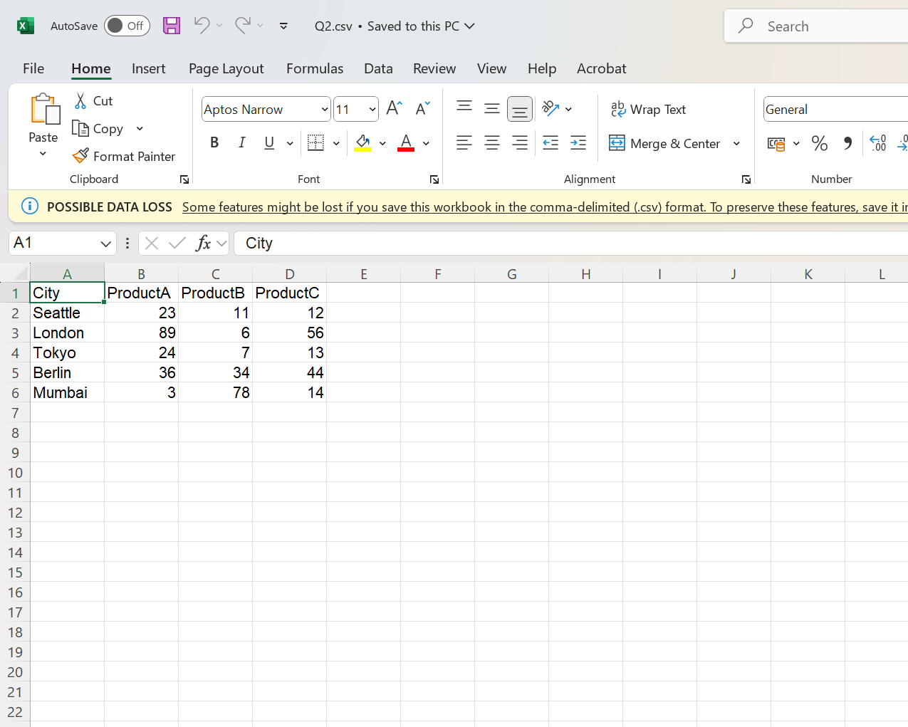
Question 2
Code
read.csv("C:\Users\TJ\R Studio\Lab 2\Q2.csv")Output
Question 3
Code
data.frame(swiss)Output
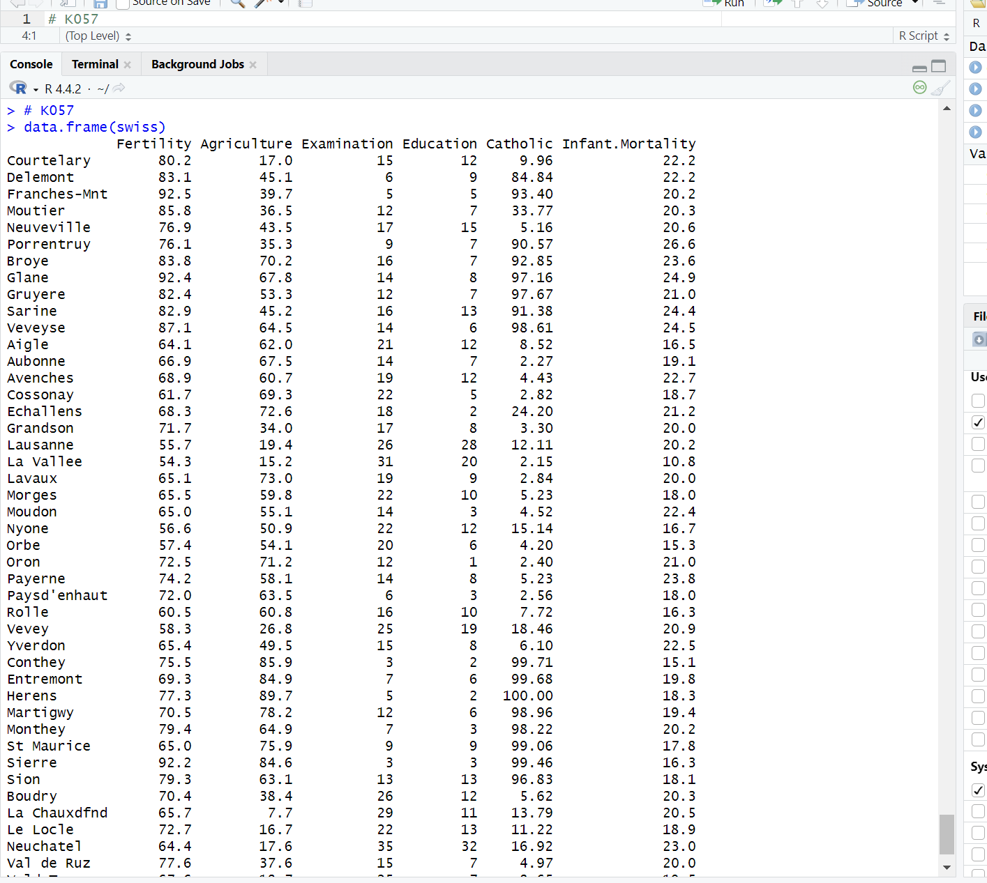
| > data.frame(swiss) Fertility Agriculture Examination Education Catholic Infant.Mortality Courtelary 80.2 17.0 15 12 9.96 22.2 Delemont 83.1 45.1 6 9 84.84 22.2 Franches-Mnt 92.5 39.7 5 5 93.40 20.2 Moutier 85.8 36.5 12 7 33.77 20.3 Neuveville 76.9 43.5 17 15 5.16 20.6 Porrentruy 76.1 35.3 9 7 90.57 26.6 Broye 83.8 70.2 16 7 92.85 23.6 Glane 92.4 67.8 14 8 97.16 24.9 Gruyere 82.4 53.3 12 7 97.67 21.0 Sarine 82.9 45.2 16 13 91.38 24.4 Veveyse 87.1 64.5 14 6 98.61 24.5 Aigle 64.1 62.0 21 12 8.52 16.5 Aubonne 66.9 67.5 14 7 2.27 19.1 Avenches 68.9 60.7 19 12 4.43 22.7 Cossonay 61.7 69.3 22 5 2.82 18.7 Echallens 68.3 72.6 18 2 24.20 21.2 Grandson 71.7 34.0 17 8 3.30 20.0 Lausanne 55.7 19.4 26 28 12.11 20.2 La Vallee 54.3 15.2 31 20 2.15 10.8 Lavaux 65.1 73.0 19 9 2.84 20.0 Morges 65.5 59.8 22 10 5.23 18.0 Moudon 65.0 55.1 14 3 4.52 22.4 Nyone 56.6 50.9 22 12 15.14 16.7 Orbe 57.4 54.1 20 6 4.20 15.3 Oron 72.5 71.2 12 1 2.40 21.0 Payerne 74.2 58.1 14 8 5.23 23.8 Paysd’enhaut 72.0 63.5 6 3 2.56 18.0 Rolle 60.5 60.8 16 10 7.72 16.3 Vevey 58.3 26.8 25 19 18.46 20.9 Yverdon 65.4 49.5 15 8 6.10 22.5 Conthey 75.5 85.9 3 2 99.71 15.1 Entremont 69.3 84.9 7 6 99.68 19.8 Herens 77.3 89.7 5 2 100.00 18.3 Martigwy 70.5 78.2 12 6 98.96 19.4 Monthey 79.4 64.9 7 3 98.22 20.2 St Maurice 65.0 75.9 9 9 99.06 17.8 Sierre 92.2 84.6 3 3 99.46 16.3 Sion 79.3 63.1 13 13 96.83 18.1 Boudry 70.4 38.4 26 12 5.62 20.3 La Chauxdfnd 65.7 7.7 29 11 13.79 20.5 Le Locle 72.7 16.7 22 13 11.22 18.9 Neuchatel 64.4 17.6 35 32 16.92 23.0 Val de Ruz 77.6 37.6 15 7 4.97 20.0 ValdeTravers 67.6 18.7 25 7 8.65 19.5 V. De Geneve 35.0 1.2 37 53 42.34 18.0 Rive Droite 44.7 46.6 16 29 50.43 18.2 Rive Gauche 42.8 27.7 22 29 58.33 19.3 |
| | | |---| |>| |
Question 4
Code
# K057

# Q4

month = c("january","february","march","december","november","january","february","march","december","november","january","february","march","december","november","january","february","march","december","november")

factor_month=factor(month)
nlevels(factor_month)
summary(factor_month)
Output
> # K057
> > # Q4
> > month = c("january","february","march","december","november","january","february","march","december","november","january","february","march","december","november","january","february","march","december","november")
> > factor_month=factor(month)
> nlevels(factor_month)
[1] 5
> summary(factor_month)
december february  january    march november
       4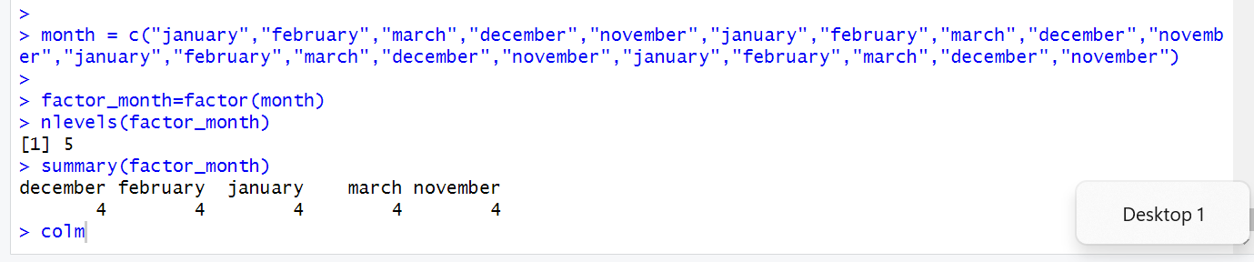
Question 5
Code
# Question 4
# K057
# Question A
# Create data frame
df <- data.frame(
Product = c("Product1", "Product2", "Product3", "Product4"),
Price = c(10, 20, 30, 40),
Quantity = c(5, 3, 6, 2)
)
print(df)
# Question B
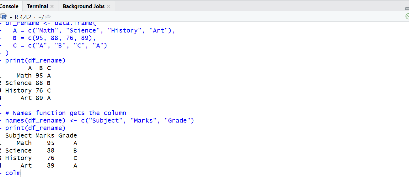
df_rename <- data.frame(
A = c("Math", "Science", "History", "Art"),
B = c(95, 88, 76, 89),
C = c("A", "B", "C", "A")
)
print(df_rename)
# Names function gets the column
names(df_rename) <- c("Subject", "Marks", "Grade")
print(df_rename)
Output
Question 6
Code
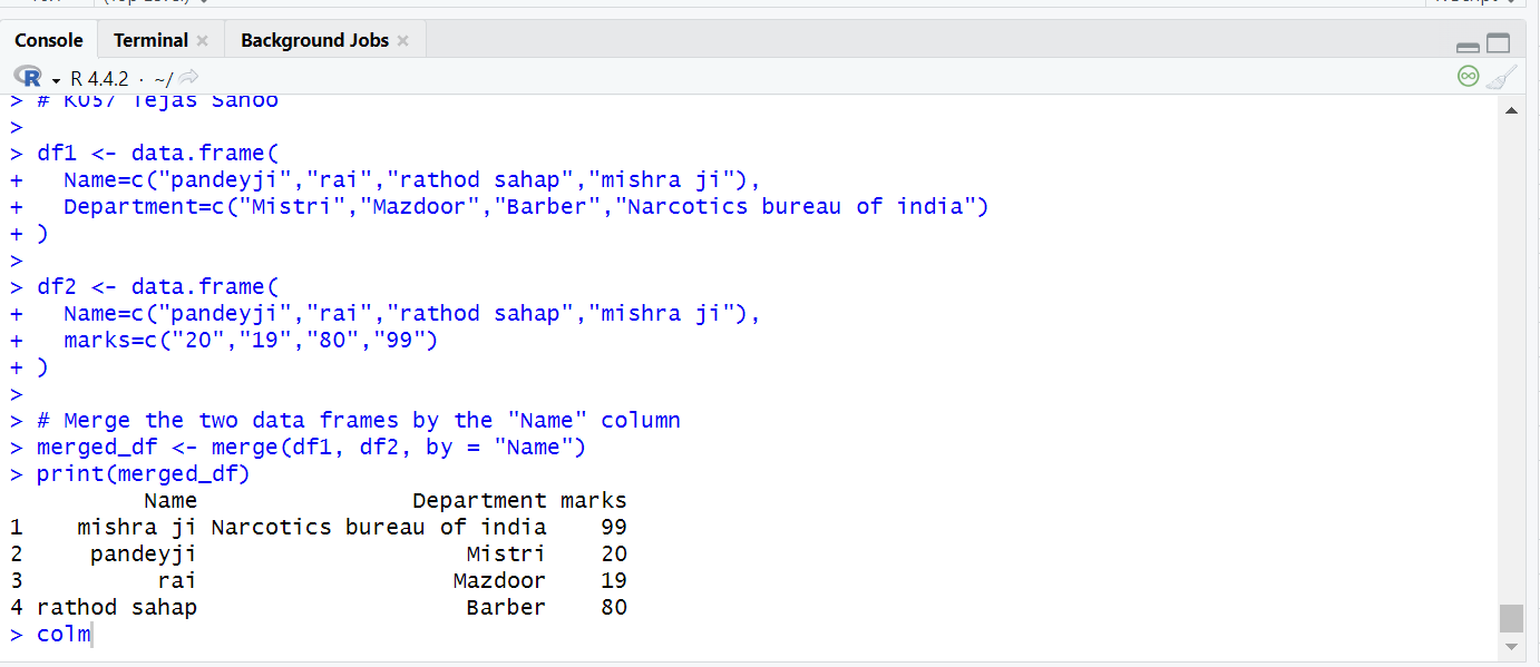
# K057 Tejas Sahoo

df1 <- data.frame(
  Name=c("pandeyji","rai","rathod sahap","mishra ji"),
  Department=c("Mistri","Mazdoor","Barber","Narcotics bureau of india")
)

df2 <- data.frame(
  Name=c("pandeyji","rai","rathod sahap","mishra ji"),
  marks=c("20","19","80","99")
)

# Merge the two data frames by the "Name" column
merged_df <- merge(df1, df2, by = "Name")
print(merged_df)
Output
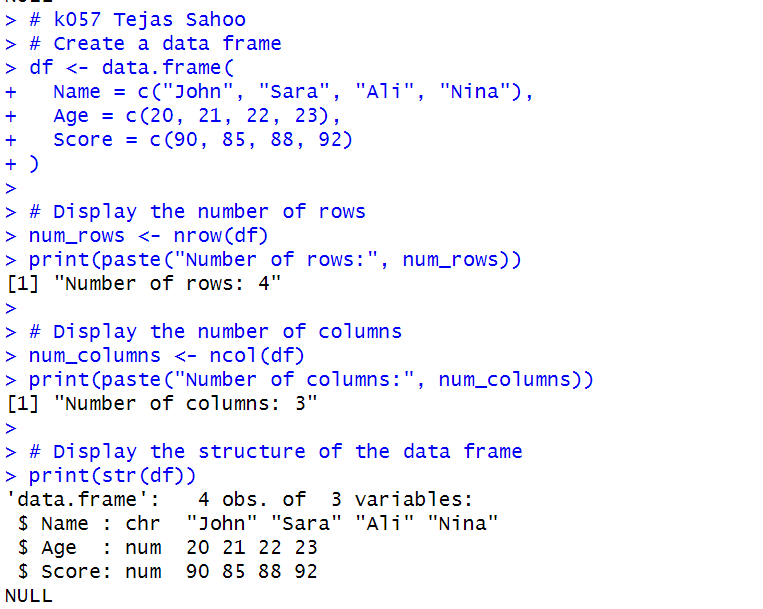
Question 7
Code
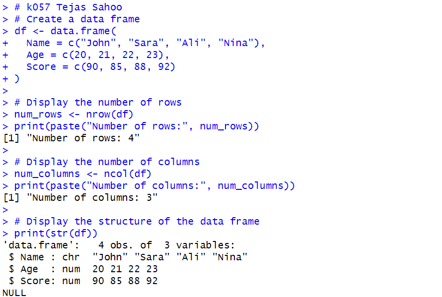
# k057 Tejas Sahoo
# Create a data frame
df <- data.frame(
  Name = c("John", "Sara", "Ali", "Nina"),
  Age = c(20, 21, 22, 23),
  Score = c(90, 85, 88, 92)
)

# Display the number of rows
num_rows <- nrow(df)
print(paste("Number of rows:", num_rows))

# Display the number of columns
num_columns <- ncol(df)
print(paste("Number of columns:", num_columns))

# Display the structure of the data frame
print(str(df))
Question 8
Code
# K057 Tejas Sahoo
Names <- c("John", "Sara", "Ali", "Nina")
Ages <- c(20, 21, 22, 23)

df <- data.frame(
  names=Names,
  ages=Ages
)

print(df)
References
Information
- date: 2025.01.10
- time: 14:48