Operating System Lab 2

Process Scheduling and FCFS

Process Scheduling

Process scheduling is a crucial component of an operating system that determines how the CPU allocates time to various processes in the system. Since multiple processes often compete for CPU time, an efficient scheduling mechanism is needed to optimize performance, ensure fairness, and maintain system stability.

Types of Scheduling

1. Long-term Scheduling:
   • Decides which processes are admitted into the system for processing.
   • Ensures the system is not overloaded.
2. Short-term Scheduling (CPU Scheduling):
   • Determines which process in the ready queue will be executed next by the CPU.
3. Medium-term Scheduling:
   • Swaps processes in and out of memory (to/from disk) to improve the execution of active processes.

---

First Come First Serve (FCFS) Scheduling

FCFS is a non-preemptive scheduling algorithm where the process that arrives first is executed first, following a simple queue structure.

---

How FCFS Works with Process Scheduling

1. Process Arrival:
   • Processes are added to the ready queue in the order they arrive.
2. Queue Execution:
   • The CPU fetches the first process in the queue, executes it, and then moves to the next one.
3. Completion:
   • Each process runs to completion before the CPU switches to the next process.

---

Advantages of FCFS in Process Scheduling

1. Simplicity:
   • Easy to implement with a straightforward logic.
2. Fairness:
   • All processes are treated equally, with execution based purely on arrival time.
3. No Starvation:
   • Every process gets CPU time eventually.

---

Disadvantages of FCFS in Process Scheduling

1. Convoy Effect:
   • A long process can block shorter ones, leading to inefficient CPU usage.
2. High Waiting Time:
   • Processes arriving later can experience significant delays.
3. Non-Preemptive:
   • Once a process starts, it cannot be interrupted, even if a higher-priority process arrives.

---

Example of FCFS in Process Scheduling

Process	Arrival Time	Burst Time	Start Time	Completion Time	Turnaround Time	Waiting Time
P1	0	5	0	5	5	0
P2	1	3	5	8	7	4
P3	2	8	8	16	14	6

Formulas:

1. Turnaround Time (TAT) = Completion Time - Arrival Time
2. Waiting Time (WT) = Turnaround Time - Burst Time AWT = (0 + 4 + 6) / 3 = 3.33 ms
   ATAT = (5 + 7 + 14) / 3 = 8.67 ms

---

Use Cases of FCFS in Process Scheduling

1. Batch Systems:
   • Ideal for systems where tasks are similar in size and priority.
2. Educational Tools:
   • Commonly used in learning environments to demonstrate the basics of scheduling.

---

Summary

Process scheduling manages how CPU time is distributed among competing processes, aiming for efficiency and fairness. FCFS scheduling, while simple and fair, is best suited for systems with predictable workloads, as it struggles with inefficiency in scenarios involving diverse process lengths. For modern multitasking systems, more advanced algorithms like Shortest Job Next (SJN) or Round Robin are often preferred.

Question

Code

 
def WaitingTime(processes, num_processes, burst_times):
    # Initialize waiting times for all processes as 0
    waiting_times = [0] * num_processes
    waiting_times[0] = 0  # First process has no waiting time
  
    # Calculate waiting time for each process
    for i in range(1, num_processes):
        # Waiting time of current process is the sum of burst time of previous process and its waiting time
        waiting_times[i] = burst_times[i - 1] + waiting_times[i - 1]
    return waiting_times
  
def TurnaroundTime(processes, num_processes, burst_times, waiting_times):
    # Initialize turnaround times for all processes
    turnaround_times = [0] * num_processes
    # Calculate turnaround time for each process
    for i in range(num_processes):
        # Turnaround time is the sum of burst time and waiting time
        turnaround_times[i] = burst_times[i] + waiting_times[i]
    return turnaround_times
 
 
def AvgTime(processes, num_processes, burst_times):
    # Calculate waiting times for all processes
    waiting_times = WaitingTime(processes, num_processes, burst_times)
    # Calculate turnaround times for all processes
    turnaround_times = TurnaroundTime(processes, num_processes, burst_times, waiting_times)
    total_waiting_time = 0
    total_turnaround_time = 0
    # Calculate total waiting time and total turnaround time
    for i in range(num_processes):
        total_waiting_time += waiting_times[i]
        total_turnaround_time += turnaround_times[i]
        print(f"\nProcess {i + 1}:")
        print(f"Burst time = {burst_times[i]} ms")  # Burst time is the time required by a process for execution
        print(f"Waiting time = {waiting_times[i]} ms")
        print(f"Turnaround time = {turnaround_times[i]} ms")
    # Calculate average waiting time and average turnaround time
    avg_waiting_time = total_waiting_time / num_processes
    avg_turnaround_time = total_turnaround_time / num_processes
    print(f"\nAverage waiting time = {avg_waiting_time:.2f} ms")
    print(f"Average turnaround time = {avg_turnaround_time:.2f} ms")
    return avg_waiting_time, avg_turnaround_time
 
  
 
print("Tejas Sahoo k057")
processes = [1, 2, 3, 4]
num_processes = len(processes)
burst_times = [21, 3, 6, 2]  # Burst times for each process which are pre defined.
AvgTime(processes, num_processes, burst_times)

To manually calculate the waiting time and turnaround time for each process in a First-Come, First-Serve (FCFS) scheduling algorithm, let’s use the given burst times and calculate the waiting and turnaround times.

Given:

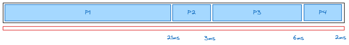
• Processes: P1, P2, P3, P4
• Burst times: [21, 3, 6, 2] (in milliseconds)

Step-by-Step Calculation:

1. Waiting Time Calculation:

• Waiting time for a process is the time it has to wait before it gets executed. For FCFS, it’s the sum of the burst times of all previous processes.

Process	Burst Time	Waiting Time Calculation	Waiting Time (ms)
P1	21	Waiting time = 0 (no previous process)	0
P2	3	Waiting time = Burst time of P1	21
P3	6	Waiting time = Burst time of P1 + P2	21 + 3 = 24
P4	2	Waiting time = Burst time of P1 + P2 + P3	21 + 3 + 6 = 30

2. Turnaround Time Calculation:

• Turnaround time for a process is the total time it spends in the system, from arrival to completion, which is the sum of the waiting time and burst time.

Process	Burst Time	Waiting Time	Turnaround Time Calculation	Turnaround Time (ms)
P1	21	0	0 + 21 = 21	21
P2	3	21	21 + 3 = 24	24
P3	6	24	24 + 6 = 30	30
P4	2	30	30 + 2 = 32	32

3. Average Waiting Time and Turnaround Time:

• Average Waiting Time = (0 + 21 + 24 + 30) / 4 = 75 / 4 = 18.75 ms
• Average Turnaround Time = (21 + 24 + 30 + 32) / 4 = 107 / 4 = 26.75 ms

Now, let’s compare this manual calculation with the output from the program.

Comparison Table (Manual vs Program Calculated):

Process	Burst Time (ms)	Manual Waiting Time (ms)	Program Waiting Time (ms)	Manual Turnaround Time (ms)	Program Turnaround Time (ms)
P1	21	0	0	21	21
P2	3	21	21	24	24
P3	6	24	24	30	30
P4	2	30	30	32	32
Average		18.75 ms	18.75 ms	26.75 ms	26.75 ms

Conclusion:

The program output matches the manual calculation. Both methods give identical results for waiting time, turnaround time, and average times. This confirms that the program works correctly for the given burst times and the FCFS scheduling algorithm.

Referenc

Information

• date: 2025.01.15
• time: 10:10